RMST Explained: Restricted Mean Survival Time for Non-Proportional Hazards in R

When the survival curves of two treatment groups cross, plateau, or separate only late in follow-up, the hazard ratio stops telling a clean story. A single hazard ratio assumes the relative risk is constant over time, and in modern oncology — especially with immunotherapies that show delayed separation — that assumption is often wrong. Restricted mean survival time (RMST) has become the standard alternative: it summarizes survival as an area under the curve, has a direct clinical interpretation in units of time, and requires no proportional-hazards assumption.
This guide explains what RMST is, why the hazard ratio breaks down under non-proportional hazards, how to choose the truncation time τ, and how to implement the analysis end to end in R with the survRM2 package (with a brief SAS equivalent). The intended reader is a biostatistician, clinical-development scientist, or regulatory reviewer who knows survival analysis but wants a precise, working model of RMST and a decision rule for when to reach for it.
What is restricted mean survival time (RMST)?
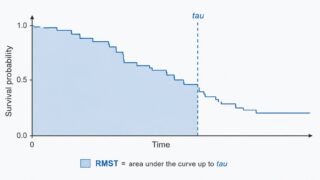
RMST is the area under the survival curve from time 0 up to a fixed time horizon τ. If \(S(t)\) is the survival function, the RMST at horizon τ is
\[
\text{RMST}(\tau) = \int_0^{\tau} S(t)\, dt .
\]
Because it integrates the survival probability over time, RMST has a concrete clinical meaning: it is the mean event-free time over the first τ units of follow-up. With overall survival as the endpoint, an RMST of 304 days at τ = 365 means that, averaged over the population, patients survive about 304 of the first 365 days. The between-group difference in RMST is then “how many extra event-free days, on average, the treatment buys over the horizon” — a quantity clinicians and patients can reason about directly, unlike a hazard ratio.
A companion quantity is the restricted mean time lost (RMTL), the area above the curve up to τ — equal to \(\tau – \text{RMST}(\tau)\). The RMTL ratio is sometimes reported alongside the RMST difference and ratio.
| Aspect | Hazard ratio (Cox) | RMST difference |
|---|---|---|
| Key assumption | Proportional hazards (constant relative risk over time) | None about the shape of the curves |
| Units | Dimensionless ratio | Time (days, months, years) |
| Clinical interpretation | Relative — “the risk is x times lower” | Absolute — “x more event-free time on average” |
| Behavior under non-PH | Ill-defined; depends on follow-up and censoring | Well-defined for any survival curves |
| Depends on | — | Choice of the horizon τ |
Why the hazard ratio breaks down: non-proportional hazards
The proportional-hazards assumption
The Cox model estimates a single hazard ratio under the assumption that the hazard functions of the two groups stay in constant proportion over the whole follow-up. When that holds, one number summarizes the effect cleanly. When it does not, the hazard ratio a Cox model reports is a hard-to-interpret average of a time-varying effect — and that average shifts with the censoring distribution and the length of follow-up, so the “same” trial analyzed at a different data cut can produce a different hazard ratio.
Three patterns of non-proportional hazards
| Pattern | What the curves do | Typical setting |
|---|---|---|
| Crossing | One group is better early, the other better later — the curves cross | Surgery vs. medical therapy with early surgical risk |
| Delayed separation | Curves overlap early, then separate | Cancer immunotherapy, vaccines |
| Converging | An early gap that narrows and closes over time | A treatment that delays rather than prevents events |
The delayed-separation pattern is the one driving the surge of interest in RMST. An immunotherapy whose benefit only emerges after several months will look unimpressive through a proportional-hazards lens — the early overlap dilutes the hazard ratio toward 1 — even though the late survival gain is real and clinically important.
Diagnosing a PH violation with cox.zph()
Before defaulting to a hazard ratio, test the assumption. In R, survival::cox.zph() performs a test based on scaled Schoenfeld residuals: a small p-value (global or per covariate) is evidence against proportional hazards, and the companion plot shows whether the effect drifts with time.
library(survival)

# NCCTG lung cancer data shipped with the survival package.
fit_cox <- coxph(Surv(time, status) ~ sex, data = lung)

# Test the proportional-hazards assumption (scaled Schoenfeld residuals).
zph <- cox.zph(fit_cox)
print(zph)      # small p-value => evidence against PH
plot(zph)       # look for a trend in the residuals over time
Read it like this: a non-significant test and a flat residual plot support reporting a hazard ratio; a significant test, a clear trend, or curves that cross or separate late are signals to summarize the effect with RMST instead. The diagnostic itself, and the alternatives to Cox when PH fails, deserve a fuller treatment of their own.
Choosing τ (the truncation time)
The one genuinely new decision RMST forces on you is the truncation time τ — the horizon over which survival is averaged. Because RMST is defined only up to τ, the choice is part of the estimand, not a nuisance parameter, and it should be pre-specified in the protocol or statistical analysis plan.
Practical guidance:
- τ must be within the observable range. A common, defensible choice is at or below the minimum of the largest observed follow-up times in the two arms. Pushing τ into a region where one arm has almost no one left at risk makes the area estimate unstable.
- Pick a clinically meaningful horizon. A 1-, 2-, or 5-year landmark that matters for the disease is easier to defend and to communicate than a value chosen purely from the data.
- Always run a sensitivity analysis over τ (see below). The RMST difference generally grows with τ when curves separate, so a single τ can over- or under-state the effect. Reporting a few horizons shows the result is not an artifact of one choice.
Pre-specify τ from clinical reasoning and the planned follow-up — not after seeing where the gap between the curves is largest. Choosing τ to maximize the observed difference inflates the type-I error in exactly the same way as any other data-driven endpoint choice.
Implementing RMST in R with survRM2
The survRM2 package implements the two-sample RMST comparison directly. Its rmst2() function returns the RMST and RMTL by arm and three between-group contrasts — the difference in RMST, the ratio of RMST, and the ratio of RMTL — and it can perform an ANCOVA-type covariate-adjusted analysis when covariates are supplied.
Data preparation
We use the NCCTG lung dataset from the survival package and compare survival by sex. rmst2() expects a 0/1 status (1 = event) and a 0/1 arm indicator, so we recode the raw lung columns (status is coded 1 = censored, 2 = dead; sex is 1 = male, 2 = female).
# install.packages("survRM2")  # first time only
library(survRM2)
library(survival)

# lung: time (days), status (1 = censored, 2 = dead), sex (1 = male, 2 = female)
dat <- lung[, c("time", "status", "sex", "age")]
dat <- na.omit(dat)

dat$status01 <- dat$status - 1   # 1/2 -> 0/1 (death = 1, censored = 0)
dat$arm      <- dat$sex - 1      # 1/2 -> 0/1 (0 = male, 1 = female)

str(dat)
'data.frame':	228 obs. of  6 variables:
 $ time    : num  306 455 1010 210 883 ...
 $ status  : num  2 2 1 2 2 1 2 2 2 2 ...
 $ sex     : num  1 1 1 1 1 1 2 2 1 1 ...
 $ age     : num  74 68 56 57 60 74 68 71 53 61 ...
 $ status01: num  1 1 0 1 1 0 1 1 1 1 ...
 $ arm     : num  0 0 0 0 0 0 1 1 0 0 ...
Unadjusted RMST comparison
Call rmst2() with the survival time, the 0/1 status, the 0/1 arm, and the horizon τ. Here we use τ = 365 days (one year).
fit <- rmst2(time   = dat$time,
             status = dat$status01,
             arm    = dat$arm,
             tau    = 365)
print(fit)
The truncation time: tau = 365 was specified.

Restricted Mean Survival Time (RMST) by arm
              Est.   se lower upper
RMST (arm=1) 304.6 14.5 276.2 333.0
RMST (arm=0) 269.4 11.8 246.3 292.5

Restricted Mean Time Lost (RMTL) by arm
              Est.   se lower upper
RMTL (arm=1)  60.4 14.5  32.0  88.8
RMTL (arm=0)  95.6 11.8  72.5 118.7

Between-group contrast (based on tau = 365)
                      Est. lower upper      p
RMST (arm=1)-(arm=0) 35.20  7.10 63.30 0.0141
RMST (arm=1)/(arm=0)  1.13  1.02  1.25 0.0179
RMTL (arm=1)/(arm=0)  0.63  0.42  0.95 0.0271
The interpretation is immediate and absolute: over the first year, females (arm = 1) survive on average 35.2 days longer than males (arm = 0), with a 95% confidence interval of 7.1 to 63.3 days and p = 0.0141. The RMST ratio (1.13) and RMTL ratio (0.63) tell the same story on relative scales. Notice that none of these numbers required a proportional-hazards assumption.
Covariate-adjusted (ANCOVA-type) analysis
To adjust for baseline covariates — say age — pass a data frame of covariates to rmst2(). The package then fits an ANCOVA-type model and reports an adjusted RMST difference (and ratios) with the covariate effects.
fit_adj <- rmst2(time       = dat$time,
                 status     = dat$status01,
                 arm        = dat$arm,
                 tau        = 365,
                 covariates = dat[, "age", drop = FALSE])
print(fit_adj)
The adjusted output adds a model table whose arm row is the age-adjusted between-group RMST contrast; read that row exactly as the unadjusted contrast above, now holding age fixed. This is the RMST analogue of adjusting a continuous endpoint with ANCOVA, and it is the version most often pre-specified as the primary analysis in a randomized trial.
Sensitivity analysis over τ
Because the RMST difference depends on the horizon, report it at several pre-specified values of τ. A short loop over rmst2() makes the trend explicit:
taus <- c(180, 270, 365)
res  <- lapply(taus, function(tt) {
  f <- rmst2(dat$time, dat$status01, dat$arm, tau = tt)
  f$unadjusted.result[1, ]   # the RMST-difference row: Est., lower, upper, p
})
do.call(rbind, res)
                       Est. lower upper      p
RMST (arm=1)-(arm=0)  14.80  1.20 28.40 0.0331
RMST (arm=1)-(arm=0)  24.60  3.50 45.70 0.0223
RMST (arm=1)-(arm=0)  35.20  7.10 63.30 0.0141
The difference grows from about 15 days at τ = 180 to 35 days at τ = 365, and stays significant throughout. A monotone, stable pattern like this is reassuring; a result that is significant at one τ but vanishes at a neighboring, equally defensible horizon should be reported as fragile.
RMST in SAS (brief)
SAS computes RMST directly in PROC LIFETEST via the rmst option, giving the same estimates and between-group difference. (As in R, specify which status value denotes censoring.)
proc lifetest data=lung rmst(tau=365);
   time time*status(1);   /* status = 1 flagged as censored */
   strata sex;
run;
Restricted Mean Survival Time (RMST), tau = 365

        sex      RMST     Std Error    95% Confidence Limits
         1     304.6        9.21         286.5    322.7      (Female)
         2     269.4        8.74         252.3    286.5      (Male)

        Difference in RMST (sex=1 - sex=2)
        Estimate    Std Error    95% CL          Chi-Square    Pr > ChiSq
          35.2        14.3      7.2  63.2           6.05         0.0139
The point estimate (35.2 days) and the between-group test (p ≈ 0.014) match the R result; small differences in the by-arm standard errors reflect the different variance estimators the two implementations use by default.
Decision flow: when to switch from Cox to RMST
RMST is not a replacement for the Cox model in every analysis — it is the right tool when the proportional-hazards assumption is in doubt. A practical sequence:
1. Fit the Cox model and test PH with cox.zph(), and look at the Kaplan-Meier curves.
2. If PH holds (flat residuals, non-significant test, no crossing), report the hazard ratio — it is an efficient, familiar summary.
3. If PH is violated, choose among the alternatives by why it failed:
– Crossing or delayed separation → RMST with a pre-specified τ gives a single, interpretable absolute effect.
– The effect of one covariate varies with time (others are fine) → a stratified Cox model or a time-dependent coefficient can keep the hazard-ratio framework.
– A consistent multiplicative model fails entirely → consider an accelerated failure time (AFT) model, which targets a time ratio.
| Situation | Recommended summary |
|---|---|
| PH holds | Cox hazard ratio |
| Curves cross or separate late | RMST difference at a pre-specified τ |
| One covariate’s effect is time-varying | Stratified Cox or time-dependent coefficient |
| Multiplicative-hazards model unsuitable | Accelerated failure time (AFT) model |
Regulatory perspective and limitations
Regulators have become increasingly receptive to RMST as a primary or key secondary summary when proportional hazards is questionable, precisely because the hazard ratio is hard to interpret in that setting and the RMST difference is not. Methodological work by Uno and colleagues and by Royston and Parmar has been influential in moving the field “beyond the hazard ratio,” and RMST sits naturally inside the estimand framework: it is a population-level summary measure for a time-to-event variable, and fixing τ is part of specifying the estimand. If you are formalizing the treatment effect of a survival endpoint, it is worth reading RMST together with the estimand attributes. See our companion article on the estimand framework and ICH E9(R1) for how the population-level summary fits with the other attributes. For continuous longitudinal endpoints the analogous workhorse is the mixed model for repeated measures — see MMRM Explained.
Limitations to keep in mind:
- τ dependence. The estimate and its interpretation are tied to the horizon. This is a feature (it makes the effect concrete) but demands pre-specification and a sensitivity analysis.
- One number over a window. RMST collapses the whole curve up to τ into a single area, so two different curve shapes can share an RMST. Always show the Kaplan-Meier curves alongside it.
- Power. When proportional hazards genuinely holds, the log-rank test / Cox model is more powerful than an RMST test; RMST’s advantage appears specifically under non-proportional hazards.
FAQ
When should I use RMST instead of the hazard ratio?
Use RMST when the proportional-hazards assumption is in doubt — crossing curves, delayed separation (as with immunotherapies), or a cox.zph() test that flags a violation. When PH holds, the hazard ratio is a fine, efficient summary.
How do I choose τ?
Pre-specify it from clinical reasoning and the planned follow-up, at or below the minimum of the largest observed follow-up times across arms, and report a sensitivity analysis over a few horizons. Never pick τ to maximize the observed difference.
Does RMST require proportional hazards?
No. RMST is defined as the area under the survival curve up to τ for any shape of curve, which is exactly why it is the standard alternative when PH fails.
What is the difference between RMST and RMTL?
RMST is the area under the survival curve up to τ (mean event-free time); RMTL is the area above it, equal to τ − RMST (mean time lost). They are two views of the same restricted window, and survRM2 reports both.
Is RMST accepted by regulators?
It is increasingly accepted as a primary or key secondary analysis in non-proportional-hazards settings, and fits cleanly into the estimand framework as a population-level summary measure. As always, confirm the intended analysis in scientific advice or a pre-submission meeting, since FDA, EMA, and PMDA expectations can differ.
Summary
The hazard ratio assumes a constant relative risk that modern survival data — crossing curves, delayed immunotherapy effects, converging benefit — frequently violate. RMST sidesteps that assumption by summarizing survival as the area under the curve up to a pre-specified horizon τ, yielding an absolute, clinically interpretable difference in event-free time. In R, survRM2::rmst2() delivers the RMST and RMTL by arm, the difference and ratio contrasts, an ANCOVA-type covariate-adjusted analysis, and (via a short loop) a sensitivity analysis over τ; PROC LIFETEST with the rmst option gives the SAS equivalent. The practical rule is simple: test proportional hazards first, keep the hazard ratio when it holds, and switch to RMST when it does not.
If you are pinning down the treatment effect of a time-to-event endpoint, read this alongside the estimand framework, where τ and the choice of summary measure are part of the estimand definition.
Further reading
- Uno H, et al. (2014). “Moving beyond the hazard ratio in quantifying the between-group difference in survival analysis.” Journal of Clinical Oncology, 32(22), 2380–2385. doi:10.1200/JCO.2014.55.2208
- Royston P, Parmar MKB (2013). “Restricted mean survival time: an alternative to the hazard ratio for the design and analysis of randomized trials with a time-to-event outcome.” BMC Medical Research Methodology, 13, 152. doi:10.1186/1471-2288-13-152
- Uno H, Tian L, Cronin A, Battioui C, Horiguchi M. survRM2: Comparing Restricted Mean Survival Time. CRAN. cran.r-project.org/package=survRM2
- Klein JP, Moeschberger ML. Survival Analysis: Techniques for Censored and Truncated Data. Springer.
- Therneau TM, Grambsch PM. Modeling Survival Data: Extending the Cox Model. Springer.