MMRM Explained: Mixed Models for Repeated Measures in R

If you analyze longitudinal endpoints in clinical trials, the mixed model for repeated measures (MMRM) is probably the single most useful tool to have a firm grasp of. It is the de facto standard for the primary analysis of continuous outcomes measured at scheduled visits — depression rating scales, lung function, pain scores, and many others — and it appears in submissions to the FDA and EMA across therapeutic areas.
This guide explains what MMRM is, why it became the default over older approaches like LOCF, how to think about its covariance structures, and how to fit it in R with the mmrm package. The intended reader is a biostatistician, clinical development scientist, or regulatory reviewer who already knows regression but wants a clear, accurate working model of MMRM.
What is MMRM?
MMRM is a likelihood-based method for analyzing a continuous outcome that is measured repeatedly on the same subjects over time. The name is slightly misleading: although it is a “mixed model,” the classic MMRM formulation used in clinical trials usually contains no random effects. Instead, it models the correlation among a subject’s repeated measurements directly, through a structured within-subject covariance matrix for the residuals.
Formally, let the vector of post-baseline measurements for subject i be modeled as a linear function of fixed effects plus correlated residuals:
\[ Y_i = X_i \beta + e_i, \quad e_i \sim N(0, \Sigma) \]
Here \(X_i\) is the design matrix of fixed effects, \(\beta\) collects the regression coefficients, and \(\Sigma\) is a covariance matrix describing how a subject’s repeated measurements vary and co-vary across time. The parameters are estimated by restricted maximum likelihood (REML), which gives less biased variance estimates than ordinary maximum likelihood.
That single idea — model the mean with fixed effects, and model the within-subject correlation with a structured \(\Sigma\) — is what makes MMRM both flexible and well suited to clinical trial data. It is best understood as the “repeated measures” special case of the broader mixed-model family, where the focus is on the residual covariance rather than on random effects.
Why MMRM in clinical trials
For decades, longitudinal trial data were often reduced to a single number per subject and analyzed with ANCOVA — most commonly the change from baseline at the final visit, with missing values filled in by last observation carried forward (LOCF). MMRM displaced that workflow for good reasons.
LOCF is a single-imputation method that distorts inference. Carrying a subject’s last available value forward treats an imputed value as if it were observed, which biases the treatment effect (in either direction, depending on the disease trajectory) and understates the standard error because it ignores the uncertainty of imputation. The 2010 National Research Council report The Prevention and Treatment of Missing Data in Clinical Trials, commissioned by the FDA, explicitly recommended against LOCF and other single-imputation approaches as a primary analysis. The EMA’s guideline on missing data in confirmatory clinical trials reached the same conclusion.
Complete-case ANCOVA wastes information. Restricting the analysis to subjects who complete the final visit discards observed data from early dropouts and is generally biased unless data are missing completely at random (MCAR) — an assumption that rarely holds in practice.
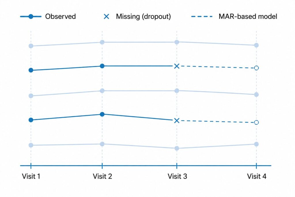
MMRM uses all observed data and is valid under MAR. Because it is likelihood-based and models every post-baseline visit jointly, MMRM includes a subject’s available measurements even if later visits are missing. Under the missing at random (MAR) assumption — that the probability of a value being missing depends only on observed data — the maximum likelihood estimates are valid without any explicit imputation. This is the property that made MMRM the preferred primary analysis under the NRC report and current regulatory thinking.
| Method | Data used | Missing-data handling | Validity / caveat |
|---|---|---|---|
| LOCF ANCOVA | Single endpoint, baseline-adjusted | Last value carried forward (single imputation) | Biased estimate, understated SE; discouraged by NRC 2010 and EMA |
| Complete-case ANCOVA | Single endpoint, completers only | Drops subjects missing the endpoint | Loss of power; biased unless MCAR |
| MMRM | All post-baseline visits jointly | All observed data via likelihood; no imputation | Valid under MAR; assumes a correctly specified mean and covariance model |
MMRM and the estimand framework (ICH E9(R1))
It is worth being precise about what MMRM does and does not decide. MMRM is an estimation method, not an estimand. The ICH E9(R1) addendum on estimands asks teams to pre-specify the target of estimation — including how intercurrent events such as treatment discontinuation are handled — before choosing an analysis method.
MMRM under MAR is most naturally aligned with a hypothetical strategy, in which the estimand reflects the outcome that would have been observed had subjects remained on randomized treatment and in follow-up. If the trial’s estimand instead calls for a treatment-policy or composite strategy, MMRM may need to be paired with a different missing-data approach, or replaced. The point is that the MAR assumption embedded in a default MMRM must be a deliberate match to the chosen estimand, not an afterthought.
The MMRM model: fixed effects, time, and covariance structures
A typical confirmatory MMRM specifies the mean structure with these fixed effects:
- Treatment (the randomized arm)
- Visit as a categorical factor — each scheduled time point is estimated separately, with no assumption of a linear time trend
- Treatment-by-visit interaction, which yields a separate treatment effect at each visit (the contrast at the final visit is usually the primary estimate)
- Baseline value of the outcome (often with a baseline-by-visit interaction)
- Stratification factors and other covariates used in randomization
Treating visit as categorical is a defining feature. It lets the treatment effect take whatever shape it actually has over time rather than forcing a parametric trajectory.
The covariance structure is the other half of the model — it tells MMRM how a subject’s repeated measurements are correlated. The choice affects the standard errors and therefore the test of the treatment effect.
| Structure | mmrm function | Parameters | Assumption | When to use |
|---|---|---|---|---|
| Unstructured (UN) | us() | t(t+1)/2 | No structure imposed on variances or correlations | Default for confirmatory trials with a small, fixed set of visits |
| Compound symmetry (CS) | cs() | 2 | Constant variance and constant correlation across all pairs | Rarely realistic for longitudinal data |
| First-order autoregressive AR(1) | ar1() | 2 | Correlation decays geometrically with the time gap; assumes equal spacing | Many equally spaced visits, when UN will not converge |
| Toeplitz | toep() | t | Correlation depends only on the lag between visits | A compromise between CS/AR(1) and UN |
Here t is the number of post-baseline time points. The unstructured matrix is the regulatory default in many programs because it makes the weakest assumptions about the within-subject correlation; the price is that it estimates the most parameters and can fail to converge with many visits or small samples. Mallinckrodt and colleagues, whose work established the modern MMRM template, recommend specifying UN first and pre-specifying a more parsimonious fallback structure in case convergence fails.
Handling missing data — why MMRM is preferred under MAR
Missing data are usually described with three mechanisms:
- MCAR (missing completely at random): missingness is unrelated to any data, observed or unobserved. Strong and usually implausible.
- MAR (missing at random): missingness depends only on observed data (e.g., earlier measurements, treatment arm, covariates).
- MNAR (missing not at random): missingness depends on the unobserved value itself, even after conditioning on observed data.
MMRM’s key property is that, as a likelihood-based method, it produces valid estimates of the mean model under MAR without explicit imputation — the likelihood for each subject is built from whatever measurements that subject actually contributed. This is why the NRC 2010 report grouped likelihood-based repeated-measures models (MMRM) and multiple imputation together as acceptable primary approaches, in contrast to single imputation.
R implementation with the mmrm package
The mmrm package (available on CRAN, maintained by the openpharma community) is the current standard for fitting MMRM in R. It is fast, supports the covariance structures above, returns Satterthwaite or Kenward-Roger degrees of freedom, and integrates with emmeans for visit-specific contrasts.
# install.packages("mmrm")
library(mmrm)

# `fev_data` ships with the package: a longitudinal trial of FEV1
# (lung function) measured at several visits, with two treatment arms.
data("fev_data", package = "mmrm")

# Fit the MMRM:
#  - FEV1 outcome
#  - treatment (ARMCD), visit (AVISIT), and their interaction as fixed effects
#  - baseline covariates (RACE, SEX)
#  - unstructured within-subject covariance, indexed by visit within subject
fit <- mmrm(
  formula = FEV1 ~ RACE + SEX + ARMCD * AVISIT + us(AVISIT | USUBJID),
  data    = fev_data,
  reml    = TRUE          # restricted maximum likelihood (the default)
)

summary(fit)
Switching the covariance structure is a one-line change — replace us() with cs(), ar1(), or toep(). Degrees of freedom are controlled by the method argument; Satterthwaite is the default, and Kenward-Roger is available for smaller samples:
fit_kr <- mmrm(
  formula = FEV1 ~ RACE + SEX + ARMCD * AVISIT + us(AVISIT | USUBJID),
  data    = fev_data,
  method  = "Kenward-Roger"
)
For the quantity most trials actually report — the treatment difference at each visit — use emmeans to obtain least-squares means and their contrasts:
# install.packages("emmeans")
library(emmeans)

# Least-squares means by arm within each visit, then the arm difference.
emm <- emmeans(fit, ~ ARMCD | AVISIT)
pairs(emm, reverse = TRUE)   # treatment minus placebo at each visit
A full worked example, from data shaping to the final-visit contrast, is covered separately.
Fitting the same model with nlme::gls
Before the mmrm package existed, the common base-R route was nlme::gls, which reproduces an unstructured MMRM by combining a symmetric correlation with visit-specific variances:
library(nlme)

fit_gls <- gls(
  FEV1 ~ RACE + SEX + ARMCD * AVISIT,
  data        = fev_data,
  correlation = corSymm(form = ~ as.integer(AVISIT) | USUBJID),  # unstructured correlation
  weights     = varIdent(form = ~ 1 | AVISIT),                   # heterogeneous variance by visit
  na.action   = na.omit,
  method      = "REML"
)
This works, but gls is slower, more prone to convergence problems, and does not offer Kenward-Roger degrees of freedom out of the box. For new analyses, mmrm is the better default; gls is mainly useful for cross-checking or in legacy code. (Note that lme4 is not a convenient choice here, because it does not directly fit an unstructured residual covariance.)
The SAS equivalent
For teams that validate against SAS, the same unstructured MMRM with Kenward-Roger degrees of freedom is:
proc mixed data=fev method=reml;
  class usubjid armcd avisit race sex;
  model fev1 = race sex armcd avisit armcd*avisit / ddfm=kr;
  repeated avisit / subject=usubjid type=un;
  lsmeans armcd*avisit / diff;
run;
The repeated statement with type=un plays the role of us(AVISIT | USUBJID), and ddfm=kr corresponds to method = "Kenward-Roger".
Interpreting the output
Reading an MMRM result comes down to a few pieces:
- Fixed-effect estimates. The coefficients on
ARMCD,AVISIT, and especially theARMCD:AVISITinteraction define how the treatment effect changes over time. Because visit is categorical, the model gives you a treatment effect per visit rather than a single slope. - The visit-specific contrast. The headline number is usually the least-squares-means difference between arms at the final scheduled visit, reported with its standard error, confidence interval, and p-value. This is what
pairs(emmeans(...))produces, and it is the estimate that typically maps to the primary estimand. - Degrees of freedom. Satterthwaite or Kenward-Roger approximations are used because the effective sample size for the within-subject covariance is not obvious. Kenward-Roger is the more conservative choice for small trials.
- Covariance parameter estimates. With an unstructured matrix these are the estimated variances at each visit and the correlations between visits — worth a glance to confirm the model converged to sensible values.
Always confirm the model converged and that the covariance estimates are plausible before interpreting the treatment effect. A non-converging UN model is the most common practical snag, which is exactly why a fallback structure is pre-specified.
FAQ
Is MMRM a mixed-effects model with random effects?
Usually not. The classic clinical-trial MMRM has only fixed effects in the mean model and captures within-subject correlation through a structured residual covariance matrix (the “R-side” covariance). It is “mixed” in the general linear-models sense, but it typically contains no random intercepts or slopes.
MMRM or ANCOVA — which should I use?
ANCOVA analyzes a single time point (often change from baseline at the endpoint) adjusting for baseline. MMRM models all post-baseline visits jointly and handles dropout under MAR without imputation. For longitudinal trials with intermittent missing data, MMRM is generally preferred; a baseline-adjusted single-visit analysis can still be reasonable when there is essentially no missing data.
Does MMRM assume MCAR, and can it handle MNAR?
MMRM is valid under the weaker MAR assumption, not just MCAR. It is not automatically valid under MNAR. For suspected MNAR, MMRM remains the primary analysis and is supplemented by pre-specified MNAR sensitivity analyses such as control-based or tipping-point multiple imputation.
Which covariance structure should I choose?
Unstructured (UN) is the usual default in confirmatory trials because it makes the fewest assumptions. If UN does not converge — common with many visits or small samples — pre-specify a fallback such as Toeplitz or AR(1). Compound symmetry is rarely a realistic description of longitudinal correlation.
Should I use the mmrm package, nlme::gls, or lme4?
Use mmrm for new analyses: it is fast, supports the standard covariance structures, and provides Satterthwaite and Kenward-Roger degrees of freedom. nlme::gls can reproduce an unstructured MMRM and is useful for cross-checking. lme4 is a poor fit here because it does not directly support an unstructured residual covariance.
Further reading
- Mallinckrodt, C. H. Preventing and Treating Missing Data in Longitudinal Clinical Trials: A Practical Guide. Cambridge University Press.
- Molenberghs, G., & Verbeke, G. Linear Mixed Models for Longitudinal Data. Springer.
- National Research Council (2010). The Prevention and Treatment of Missing Data in Clinical Trials. The National Academies Press.
- ICH E9(R1) (2019). Addendum on Estimands and Sensitivity Analysis in Clinical Trials.
Looking for a structured path through longitudinal modeling and missing-data methods for clinical trials? A focused course can be a faster way to build fluency.